By: Marc Lombardo
2020 and the Question of Aerosol Cooling
While 2020 was not incontestably the warmest year on record globally—measurements have it as being marginally cooler than 2016, though this was within the margin of error—it was demonstrably the warmest year ever experienced in the Northern Hemisphere. And, unlike 2016, which was an intensely strong El Nino year, 2020 started off as ENSO-neutral and after September actually had a La Nina influence. I cannot help but wonder if the unexpectedly high temperatures of 2020 may be evidence of something other than simply the logical result of ever-increasing greenhouse gas levels in the atmosphere. Of course, one factor that distinguished 2020 from all other years was the temporary reduction in anthropogenic fossil fuel emissions (particularly in the Northern Hemisphere) due to the Covid Lockdown.
Figure 1.1
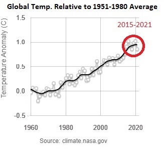
Figure 1.2
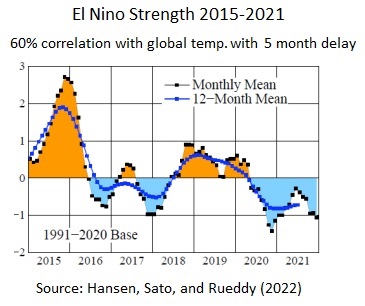
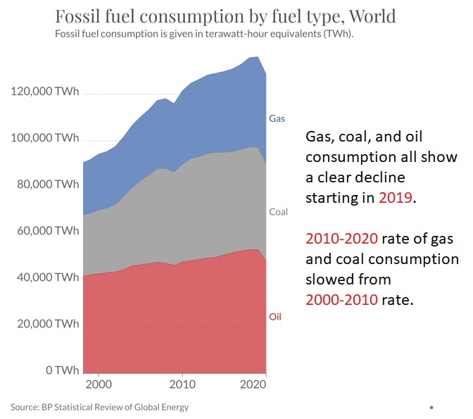
Figure 1.3
Measuring the temporary cooling effect produced by the impact of aerosol particles from anthropogenic emissions upon albedo is among the most controversial and important questions for any attempt to mitigate the effects of anthropogenic climate change. Bellouin et al. (2020) tried to narrow the range of estimates for the total effective radiative forcing of aerosols and came up with a window of -1.6 to -0.6 W m−2 with a 68% confidence interval and -2.0 to -0.4 W m−2 with 90% confidence; or, as they say in the plain language summary, the total cooling effect of aerosols “offsets between a fifth and a half of the radiative forcing by greenhouse gases.” Using satellite observations, Jia, et al. (2021) found total observed aerosol radiative forcing to be −1.09 W m−2—more or less right in the middle of the range provided by Bellouin et al. (2020)—but with a 133% stronger observed cooling effect over land than was previously estimated. When we compare these recent figures for aerosol cooling with the estimated radiative forcing from anthropogenic emissions alone (~2.1 W m−2 in 2020), the phenomenon appears to offset a bit more than half of human-derived warming. Lelieveld, et al. (2019) find that:
“fossil-fuel-related emissions account for… 70% of the climate cooling by anthropogenic aerosol… Since aerosols mask the anthropogenic rise in global temperature, removing fossil-fuel-generated particles liberates 0.51(±0.03) °C… The largest temperature impacts are found over North America and Northeast Asia, being up to 2 °C. By removing all anthropogenic emissions, a mean global temperature increase of 0.73(±0.03) °C could even warm some regions up to 3 °C.”
While these contemporary findings on aerosol cooling are by no means negligible in their effect size, they are actually somewhat lower than the aerosol-derived cooling effect that Hansen et al. (2011) estimated for 2010 of -1.6 ± 0.3 W/m−2. Hansen believes that the decline in measured aerosol cooling over recent years compared with prior estimates reflects a true change in the phenomenon rather than simply a refining of measurements. Referencing the accelerated warming trend evident in the 2015-2020 period, Hansen, Sato, and Rueddy (2022) write: “that accelerated warming seems to be caused by a decrease of human-made aerosols; the moderately increased growth rate of greenhouse gases (GHGs) in the past several years cannot account for the observed large increase of Earth’s energy imbalance.” Comparing the three charts above shows that the abrupt 2015-2020 global temperature increase cannot be explained by ENSO states or fossil fuel consumption.
Not only did the period from 2015-2020 see a dramatic acceleration of global warming. During this same period, the number of extreme weather events in the US also greatly increased. The National Centers for Environmental Information reports the following regarding the more frequent occurrence of extreme weather events in the US resulting in destruction totaling over a billion dollars: “The 1980–2021 annual average is 7.4 events (CPI-adjusted); the annual average for the most recent 5 years (2017–2021) is 17.2 events (CPI-adjusted).” Could this dramatic increase in highly destructive extreme weather events in the US over recent years possibly be related to the decreased cooling from aerosol radiative forcing that Hansen surmises to have taken place over the same period?
Mann et al. (2018) offered a global simulation showing that in the long run lower aerosol levels could lead to fewer extreme weather events, despite temperature increases, but even if this holds as a global trend, there may be contrary effects on particular regions. Looking at disasters globally, the UN Office for Disaster Risk Reduction did find that the number of disasters during the 2010s actually declined from the 2000s; nevertheless, they also project global disasters to exceed 2000s levels in the near-term: “If current trends continue, the number of disasters per year globally may increase from around 400 in 2015 to 560 per year by 2030”. While recent global disaster trends remain somewhat murky, this is not the case for the US as a region. When aerosols were at their lowest levels in recent memory in the US during the year of 2020 thanks to the Covid Lockdown, there were “22 separate billion-dollar weather and climate disasters across the United States, shattering the previous annual record of 16 events, which occurred in 2017 and 2011.”
In recent interviews, Michael Mann acknowledges the cooling impact of aerosols but argues that the removal of this cooling can be regarded as a modest tax upon efforts to reduce greenhouse gas emissions. Even if Mann’s 2018 hypothesis that lower aerosol levels would drive fewer extreme weather events was correct globally and over a longer time scale than recent events such as the Covid Lockdown allow us to observe, it is still unclear that the calculus regarding the impact of human-derived aerosols upon global temperature is as straightforward as Mann presents. While it is indeed certain that the cooling effect of anthropogenic aerosols is significantly less than the total positive radiative forcing of present levels of greenhouse gases, changes to anthropogenic emissions cannot possibly reduce GG radiative forcing entirely. For one thing, there are and will continue to be significant non-anthropogenic sources of carbon emissions. For instance, Xu et al. (2020) find that “From 1997 to 2016, the global mean carbon dioxide emissions from wildfires equated to approximately 22% of the carbon emissions from burning fossil fuels.” More concerning still is the fact that any efforts taken to reduce emissions now will have little to no discernible cooling effect upon global temperature for decades.
Mann has widely proclaimed the IPCC’s model of decarbonization that posits a steady decline in global temperature 3-5 years following the introduction of a net-zero emissions regime. However, this model is at considerable variance with other estimates. For instance, Samset, Fuglestvedt, and Lund (2020) find that there would be no measurable reduction in the rate of global temperature increase for 21 years following the implementation of a net-zero emissions regime. Evidently, this variance in projections arises as a result of differing views on how the carbon cycle will respond to emissions reductions. According to Mann, if humans were to “stop emitting carbon right now … the oceans start to take up carbon more rapidly” (Mann quoted by Hertsgaard, 2020). Mann claims that this prediction is a result of “new science” that even he was unaware of until recently—and he only cites the IPCC’s 6th report for this claim rather than any primary sources—however, it’s difficult to see how the record of air-sea carbon flux supports this prediction. While there is some interannual and decadal variability in air-sea carbon flux largely having to do with ENSO states and other varying circulation patterns, the overall trend for the last 60 years is beyond clear: ocean carbon uptake has increased largely in parallel with atmospheric carbon increases (Bennington, Gloege, McKinley, 2022; Friedlingstein et al., 2021). Why would we expect this long-standing trend to abruptly reverse?
Upon reviewing estimates for the total amount of carbon presently in the atmosphere and the maximum possible rate at which atmospheric carbon could conceivably drawdown into ocean and land sinks, the decarbonization claims of Mann and the IPCC are difficult to fathom without the introduction of some unknown deus ex machina of remarkable effect. Increases in GG emissions, atmospheric carbon levels, and ocean + land carbon uptake have tracked closely over the past six decades during which we have the best data.
Figure 1.4
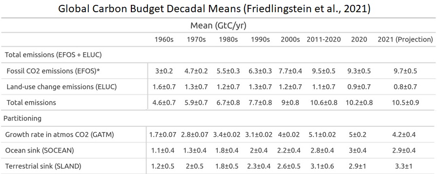
What amount of carbon drawdown would it take to slow GG warming to 1990 levels (which is to say nothing of stopping GG warming entirely, as Mann and the IPCC posit is possible in as little as 3-5 years)? Ostensibly, we would need to draw atmospheric C02 back to ~350 ppm, as Bill McKibben has so vociferously insisted for so long, i.e., a total of roughly 750 GtC of atmospheric carbon. NB: this total is still at least 90 GtC above pre-industrial. Even if we assume the highest plausible rate of ocean and land uptake (the 2021 projected rate of 6.2 GtC/year plus the maximum possible error of +1.4 GtC/year) as a constant 7.6 GtC/year, given that total atmospheric carbon at present is ~900 GtC, it would take 20 years of net-zero emissions to return us to 350 ppm; and note that this most optimistically plausible estimate very closely agrees with the results of Samset, Fuglestvedt, and Lund (2020) who found that it would take 21 years of net-zero to result in any measurable slowing to the rate of global warming. Assuming a more likely scenario in which the drawdown of atmospheric carbon starts from 6.2 GtC/year (the mean 2021 projection) and decreases linearly to 1990s levels—after all, historically, oceans and lands store carbon at higher rates when it is present in the atmosphere at higher rates—it would instead take 29 years of net-zero emissions for atmospheric CO2 to return to ~350 ppm. The decarbonization timeline of Mann and the IPCC seems off by a factor of no less than 4 and up to an order of magnitude.
In any event, what is undoubtedly clear is that GG warming and aerosol cooling take place on radically different time scales. Some portion of carbon dioxide emitted now will continue to cycle through the climate system for thousands of years, whereas cooling aerosols fall down to the ground within days. The significance of this fact is that any efforts to reduce carbon dioxide emissions that also reduce aerosols will by definition result in temperature increases in the short-term. Anyone who proposes cuts to carbon emissions but who does not acknowledge the short-term global temperature increase such a project would cause as a basic fact of atmospheric physics does the field of climate science a much greater disservice than the most oblivious or disingenuous of climate change deniers could ever dream.
Moreover, if the short-term temperature increases resulting from lowering anthropogenic emissions in turn drive positive feedback cycles—e.g., more numerous and larger wildfires, greater release of permafrost-sequestered methane, decreased albedo from loss of glacial ice, a collapse of the gulf stream system, etc.—this would further reduce (and may even trump) any possible long-term cooling from lowering carbon dioxide emissions. One well-understood feedback amplification mechanism that must be considered is the increased atmospheric water vapor that follows from temperature increases. Ramanathan and Inamdar (2009) find that for every 1 degree K increase in global temperature, water vapor contributes an additional positive radiative forcing of 1.42 W m−2 and does so on a much more rapid time-scale than any possible cooling from emissions reductions. The authors conclude that the full force of water vapor feedback will be evident within the course of a single year at the latest.
The Covid Lockdown provided the largest reduction in greenhouse gas emissions in the period for which we have highly resolved data and thus our first major opportunity to assess the immediate real-world climate impacts of anthropogenic GG emissions reductions. Gettelman et al. (2021) examined the effect of the 2020 Lockdown upon global temperature and found the peak ~20% reduction in anthropogenic greenhouse gas emissions to have at its maximum impact led to ~.15 degree C of warming averaged across the globe and a ~.35 degree C increase over the landmasses of the US and Russia. This finding comports surprisingly well with the estimate of Lelieveld, et al. (2019) that the total loss of short-term cooling from anthropogenic emissions would produce a total near-term warming of 0.73(±0.03) °C as a global mean. Using the findings of Ramanathan and Inamdar (2009) regarding the positive feedback cycle of water vapor and temperature increases, the .73°C global estimated temperature increase from the loss of anthropogenic emissions would in turn result in an additional 1.04 W/m−2 of positive radiative forcing from the added water vapor in the atmosphere alone. Thus, it appears that the combination of the loss of aerosol cooling and the associated increase in water vapor would in and of itself be enough to obliterate the long-term cooling that is supposed to accompany reductions in anthropogenic emissions.
Let us consider the rate of temperature increase that we would expect to follow from this net-zero emissions scenario. Loeb et al. (2021) estimated the magnitude of Earth’s energy imbalance to be 1.12 ± 0.48 W m−2 in mid-2019—a quite dramatic increase from the estimated value of 0.42 ± 0.48 W m−2 in mid-2005. Getting rid of the temporary cooling from anthropogenic emissions would approximately double the present imbalance in the course of a week; the additional positive forcing from water vapor at the resulting higher temperature would in turn almost triple the energy imbalance in the course of a year. A conservative measure of the present decadal rate of global temperature increase is .22 C/decade (using the 1990-2020 average). The .22 C/decade rate observed from 1990-2020 is almost certainly an underestimate of the present rate of global warming as the observed increase from 2010-2020 was .394 C/decade. Nevertheless, we will keep .22 C/decade as our lower bound to account for any negative feedback due to the presumed drawdown of atmospheric carbon following net-zero discussed above. Adding the loss of aerosol masking (1.09 W/m−2) and the accompanying forcing from water vapor (1.04 W/m−2) to the present energy imbalance would in turn imply a minimum global temperature rate increase of .532 – 1.47 C in the decade following net-zero. This range of decadal temperature increase should be regarded as an absolute minimum to follow from the onset of net-zero in that this rate does not include any other of the numerous possible positive feedbacks that may well be triggered at the implied temperatures.
Even using the bottom end of this estimate for the rate of global temperature increase following the onset of net-zero emissions—almost certainly an underestimate, given the high agreement between the prediction of Lelieveld et al. (2019) of a .73 C increase to follow immediately from the loss of anthropogenic emissions and the observed increase of .15 C that followed the ~1/5th reduction of emissions evident during the Covid Lockdown, to say nothing of the water vapor feedback—the planet would blow past the IPCC’s target of 1.5 C above the 1850-1900 average in only a handful of years. In a scenario near the mean of this potential rate increase (1C / decade), we would experience the perils of a +2C world that the IPCC warns of in the decade following net-zero implementation: 37% of the global population would be subjected to extreme heat once every five years, wildfires will burn 35% more area annually than at present, 12-29% of species would be at high risk of extinction, and as many as 3 billion people may experience water scarcity. A scenario near the high end of the estimated temperature rate increase (1.47 C/decade) following net-zero emissions, which certainly cannot be ruled out given that the observed temperature rate increases of each of the past 4 decades have exceeded the linear projections from the decade before even without the additional forcing from a total loss of aerosols, would lead us to a near-term future that in all likelihood would be beyond the scope of our species’ adaptive abilities.
Due to the carbon drawdown timeline discussed above, we should not expect the rate of global warming to slow for at least two decades following the onset of net-zero, but when we look closer at the relevant factors, it seems that this estimate seems unduly optimistic. Following upon this timeline, were we to implement net-zero tomorrow, we would already be committed to a world that is at least ~2.3 C above pre-industrial as the absolute best-case scenario 20 years after implementation. This figure was obtained by adding the lower bound increase to the Earth energy imbalance for 20 years after net-zero (.532 C /decade x 2 = 1.064 C) to the averaged 2016-2020 yearly global temperature anomaly relative to 1850-1900 (1.22 C).
However, over this longer time scale, we also need to add an additional positive feedback from water vapor not accounted for in the change to the Earth energy imbalance to follow in the short-term from net-zero. At +2.3 C, the positive radiative forcing from water vapor would be an additional .47 W m−2 above that used in the EEI estimate for a total of 1.51 W m−2 above present and 3.27 W m−2 above 1850-1900 baseline. Even assuming that greenhouse gas radiative forcing miraculously declines to its 1990 level (~2.2 W m−2 above pre-industrial, that is, a decline of ~1 W m−2 from present levels) by the time period in question—i.e., 20 years after the onset of net-zero—the Earth energy imbalance would still be between 1.15 and 2.11 W m−2 at that point (this wide range owing to the uncertainty in the present EEI estimate). In other words, assuming the fastest plausible drawdown of atmospheric carbon, far from global temperature starting to decline 20 years after the implementation of net-zero, we should expect the rate of temperature increase to be unchanged from what it is at present as an absolute best-case scenario.
Of course, the idea of anthropogenic emissions falling to zero overnight is a distant fantasy (and, some believe, a problem that we wish we had). Nevertheless, the clear decoupling of the trend of increasing temperature with anthropogenic emissions that is evident since 2015 suggests that even modest reductions in human usage of the most polluting fuels can have very significant near-term real-world consequences. In popular discussions about moving to a carbon neutral economy, the short-term warming associated with reduced pollution particulates in the air is rarely mentioned, but the findings discussed above suggest that the loss of short-term cooling from anthropogenic emissions would likely spur feedbacks capable of offsetting (and possibly trumping) any gains made from eliminating anthropogenic GG emissions. When we consider that the aerosol cooling effect is immediate, loss of any significant portion of that cooling at a given moment in time may well be sufficient to cause near-term increases in temperature capable of pushing the Earth beyond pivotal climate tipping points such as the elimination of Summer arctic sea ice. Even in the extremely unlikely event that the cumulative global impact of reduced air particulates upon temperature is relatively low, we may still see a more dramatic impact upon the populated areas that emit the bulk of pollutants. Might such an impact be enough to trigger extreme temperature events capable of stressing infrastructure, decimating crop yields, and/or compromising human health in particular regions at particular times?
Tucson’s Unbelievably Hot Summer 2020: A Case Study
I wonder if there is not a way of analyzing the record-breaking heat we experienced during Tucson’s Summer of 2020 so as to view the unique conditions that prevailed here over those months as a kind of natural experiment into the local impacts of losing a significant amount of the temporary cooling from anthropogenic emissions. In 2020, Tucson recorded its hottest May, July, August, and September ever in terms of average temperatures; May and August also both recorded their hottest average highs as well. Using data from 1991-2021, while the May 2020 average was not quite statistically significant (p = .0668), July 2020 (p = .0202), August 2020 (p = .0023), and September (p = .0401) all clearly were. I’m not sure of the best method for calculating the combined probability of these events given that there is some degree of correlation between them and so they are not truly independent, but I am quite sure that the result would stand out as highly significant, even in contrast to the clear overall warming trend from 1991-2020. Here’s the formula that I used:
(Month A – Month B Correlation) (Z-score Difference of Observed A 2020 from Projected A 2020) (STDEV of B) + Projected 2020 B from trend = Total Expected B 2020
For July, August, and September, I then averaged the totals from this formula for all of the relevant monthly pairs. That is, for August, the total temperature (in F) correlation adjustment added to the linearly projected August temperature averages the formula results for the May-August and July-August pairs. Utilizing this method, we get the following results:
May – Projected 2020 from Trend = 76.886 F, Observed 2020 = 80.7 F, Z-score of difference of observed from projected May 2020 = 1.428 , p = .0764
July – Projected 2020 = 88.545 F, correlation between May and July (.119) times May 2020 Observational Difference Z-score (1.428) times July STDEV (1.698) = Total Expected July 2020 = 88.834 F, Observed July 2020 = 91.5 F, July 2020 Z-score difference obs. Vs. total expected = 1.57 = p of hotter July 2020 than observed given May 2020 and trend = .0582
August – Projected 2020 August = 87.525 F, Correlation between May and August (-.14521) times May Z-score differential (1.428) times Aug STDEV (1.877) = -.389, Correlation July and August (.394547) times July Z-score differential (1.57) times Aug STDEV = 1.163, Average correlation adjustment of Aug 2020 = .387 F, Total Expected August 2020 = 87.912 F, Observed 2020 = 92 F, 2020 August Z Differential = 2.178 = probability of hotter August 2020 than observed given May and July 2020 and trend = .0146
September – Projected 2020 September = 83.204, Correlation between May and September (.142347) times May 2020 Z-score differential (1.428) times September STDEV (1.727) = .351, Correlation between July and September (.187376) times July 2020 Z-score differential (1.57) times September STDEV (1.727) = .508, Correlation between August and September (.3557) times August 2020 Z-score Differential (1.971) times September STDEV (1.727) = 1.211, Combined Averaged Correlation adjustment for September 2020 = .69 F. Total Expected 2020 September = 83.894 F, Observed 2020 September = 85.7 = 2020 Z Differential = 1.046, probability of hotter September 2020 than observed given trend and observed May, July, and August 2020 = .1469
Combined probability of May, July, August, and September all hotter than observed 2020 given trend = 0.0000095365435152
The co-occurrence of these four record hot months over the same Summer is a signal worthy of notice unto itself but intuitively it also raises the question: what about June? As I’ve already mentioned, June was the only month during Tucson’s Summer 2020 that did not have the hottest average for the month on record, though it was still .225 degree above the 1991-2021 average, making it the 17th warmest June on record. Still, this was actually quite a bit lower than the temperature for June 2020 that one would expect given the ongoing warming trend and the observed temperatures of May 2020:
Projected June 2020 from trend = 88.08 F + May-June Correlation (.159004) times May 2020 Differential Z-score (1.428) times June STDEV (2.33) = Total Expected June 2020 = 88.609 F, Observed June 2020 = 86.4 F, June 2020 Observed vs. total expected differential Z-score = -.948, probability of a June cooler than June 2020 given May 2020 and trend = .1711
In other words, the observed average temperature of June 2020 was a full 2.2 degrees cooler than what you would expect from the ongoing warming trend and after observing May 2020. For this result to be compatible with the hypothesis of 2020’s Summer temperatures being driven to new heights due to the emissions reductions of the Covid Lockdown, some other factor would need to have been at play that made June 2020 so different from the other months of Summer 2020. There was in fact something quite different about June from the perspective of the aerosol masking effect. The National Weather Service writes:
“The main story of the month was the Bighorn Fire on the Catalina mountains which was started by a lightning strike on Pusch Ridge on the 5th. Over 118,000 acres has burned at the close of the month with 54% containment and ranks as the 8th largest wildfire in Arizona so far on record. For reference the Aspen Fire in 2003 burned 84,750 acres and ranks as the 9th largest wildfire in Arizona on record.”
Just like anthropogenic fossil fuel emissions, wildfires contribute a significant amount of both greenhouse gases and aerosols to the atmosphere. The latter can produce a quite dramatic short-term cooling effect upon regional surface temperatures. For instance, looking at the 2019-2020 Australian wildfires, Chang et al. (2021) found that “wildfire-derived air pollution was associated with an aerosol optical thickness of >0.3 in Victoria and a strongly negative ARF [aerosol radiative forcing] of between −14.8 and −17.7 W m−2, which decreased the surface air temperature by about 3.7 °C–4.4 °C.”
Here then is the story of Tucson’s Summer 2020 that only slowly came into focus for me but that I can no longer unsee: directly following the reduction of fossil fuel emissions from lockdown restrictions, Tucson experienced its hottest May ever recorded. Hot summer temperatures are known to bring together thunderstorms here, which in this case, coming earlier in the season and in a much drier overall weather pattern, resulted in the worst fire in the state of Arizona in a generation. The Bighorn Fire took place in the mountains directly above Tucson and its huge plumes of smoke blocked out much of the sun that would have doubtless otherwise blasted us here for the month of June. Whereas the Bighorn Fire burned 118,000 acres in June, the fire was significantly contained by the end of the month such that less than 2,000 additional acres burned in July.
Lower-than-expected June temperatures gave way to much higher than expected July temperatures, just as the aerosol masking effect hypothesis would predict. And this is despite the fact that there was still likely some residual cooling influence from the Bighorn Fire upon July 2020 temperatures. With the Bighorn Fire’s plumes of smoke largely dispersed to the East and without their yet being replaced by the typical amounts of aerosols from tailpipes and smokestacks thanks to the Covid Lockdown—Liu et al. (2020) show that unlike in China and many European countries, emissions reductions due to lockdown continued in the US through the Fall of 2020—this set the stage for the truly exceptional temperatures of August 2020.
Cumulatively, we see that following the introduction of the Covid Lockdown, temperatures rose well above expectations in May, only to decline below our expectations when a new source of emissions was introduced in June (the Bighorn Fire), only to climb again once the plumes of smoke dissipated in July and, most significantly, August. Rather than disputing the hypothesis, given that June 2020’s lower than expected temperatures were likely due to an abundance of fire-derived aerosols, the June temperature observations actually support the hypothesis that the absence of aerosol cooling is the likely cause of 2020’s unexpected warming in Tucson.
This hypothesis raises more questions than it answers: How can it be effectively demonstrated that no other factors exerted a substantial causal influence upon Tucson’s Summer 2020 temperatures? Is the aerosol masking effect a more dramatic phenomenon in Tucson than in other generally less dry and more cloudy regions and is that why many other regions did not experience similar temperature spikes during Summer 2020? Supposing the aerosol masking hypothesis is a correct explanation of 2020 for our dusty little town, to what extent can these results be generalized to other regions and other times? Moreover, can a fuller appreciation of the regional cooling effect of aerosols lead to more accurate predictions of the regional temperature effects of changes in anthropogenic GG emissions? The latter question may prove immediately relevant as the conflict in Ukraine pushes global fuel prices to points that will likely lead to reductions in usage.
Likelihood of Tucson Summer 2020 Events when Including June as Supporting Hypothesis
May – Projected 2020 = 76.886 F, Observed 2020 = 80.7 F, Z-score of difference of observed from projected May 2020 = 1.428 , p = .0764
June – Projected June 2020 = 88.08 F + May-June Correlation (.159004) times May 2020 Differential Z-score (1.428) times June STDEV (2.33) = Total Expected June 2020 = 88.609 F, Observed June 2020 = 86.4 F, June 2020 Observed vs. total expected differential Z-score = -.948, probability of a June cooler than 2020 given May 2020 and trend = .1711
July – Projected 2020 = 88.545 F, correlation between May and July (.119) times May 2020 Observational Difference Z-score (1.428) times July STDEV (1.698) = .289, Correlation between June and July (.06) times June 2020 Z Difference (-.948) times July STDEV (1.698) = -.097, Average Correlation Adjustment = .096 F = Total Expected July 2020 of 88.641, Observed = 91.5, Z Difference = 1.684, p = .0465
August – Projected 2020 August = 87.525 F, Correlation between May and August (-.14521) times May Z-score differential (1.428) times Aug STDEV (1.877) = -.389, Correlation between June and August (.092693) times June Z Differential (-.948) times Aug STDEV (1.877) = -.165, Correlation between July and August (.394547) times July Z Differential (1.684) times Aug STDEV (1.877) = 1.247, Averaged Correlation Adjustment = .231 = Total Expected August 2020 = 87.756, Observed = 92, Z Difference = 2.261, p = .0119
September – Projected 2020 September = 83.204, Correlation between May and September (.142347) times May 2020 Z-score differential (1.428) times September STDEV (1.727) = .351, Correlation between June and September (-.08012) times June 2020 Z Difference (-.948) times September STDEV (1.727) = .131, Correlation between July and September (.187376) times July 2020 Z Differential (1.684) times September STDEV (1.727) = .545, Correlation between August and September (.3557) times Aug 2020 Z Differential (2.261) times September STDEV (1.727) = 1.389, Averaged Correlation Adjustment = .604 = Total Expected September 2020 = 83.808 F, Observed = 85.7 F , Z Difference = 1.096, p = .1357
Combined total probability = 0.0000009815741894238
History of Tucson Summer Heat Anomalies 1950-2021
As hot as Tucson’s Summer 2020 certainly was, in all likelihood, it would have been much hotter without the influence of the Bighorn Fire. Moreover, tracking the history of Tucson summer heat anomalies with significant deviations from the overall warming trend allows us to consider the likelihood of an even more anomalous heating event than Summer 2020. While 2020 was incontestably the hottest summer in Tucson’s history in terms of raw temperatures, due to the lower-than-expected temperatures of June 2020, it was actually only the second most anomalously hot summer as compared to the underlying warming trend.
Figure 2.1
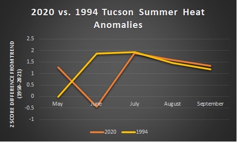
As a useful point of comparison, let’s look at the third most anomalously hot summer in Tucson between 1950-2021, which occurred way back in the year 1952.
Figure 2.2
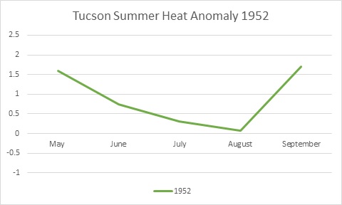
With the exception of 2020’s plummeting June temperatures, quite likely due to the aerosol influence of the Bighorn Fire, the Summers of 1994 and 2020 have similarly shaped bell curves with May and September being less anomalous than the middle months. This is the inverse of the U-shaped curve for 1952, which is a more extreme form of the typical weather pattern for the region, due to the flattening influence of the July-August monsoons. By contrast, the example of 1994 shows what can happen to the region’s summer temperatures when the monsoon rains don’t come.
Figure 2.3
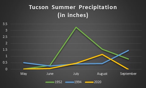
Tucson’s Summer 1994 actually started with a half inch of rain, which may not sound like a lot to those from wetter climates, but that’s actually slightly above the region’s average May rainfall and, unsurprisingly, May ’94 temperatures were slightly below trend. However, the mid-summer months of 1994 (June, July, August) were together the driest on record, and correspondingly, the temperatures of those months for 1994 also showed the greatest combined positive deviation from trend ever observed for those months.
2020 had almost no rain whatsoever for May, June, or September and so when one counts the overall precipitation from May to September it was the driest summer in Tucson’s history. Nevertheless, the traditional monsoonal pattern of July-August was faintly perceptible in 2020, culminating in over an inch of rain for August and making it only the 15th driest August from 1950-2021. However, despite Tucson receiving over .7” more rain during August 2020 than August 1994, and despite the -.45 correlation between precipitation and temperature for the month of August during 1950-2021, the temperature anomaly of August 2020 was even greater than that of 1994. Not only does this collection of facts provide evidence for the impact of the loss of aerosols upon August 2020 temperatures; to my mind, it also raises the question of what a summer as dry as 1994 and with even fewer aerosols than 2020 would look like. Fire may well be the climate’s endogenous negative feedback mechanism in response to escalating temperatures, but this negative feedback is not infinitely elastic in response to greater and greater stresses. This phenomenon is not dissimilar to the manner in which your home air conditioner will keep you at a balmy 72 F until all of a sudden, one day, it doesn’t work at all—having shown few if any prior signs of imminent collapse aside from a few unusual electrical groans and whimpers that can be easily ignored until it finally actually stops working.
It’s Not Averages that Kill, it’s Extremes
Compiling and comparing average temperatures such as was done above can be a useful and hopefully illuminating statistical exercise, but the extremes are where the rubber meets the road with respect to the question of preserving habitat for living creatures (including homo sapiens). Regardless of whatever the average temperature may be for a given region for a given year or season, a single day that is hot enough can present a challenge to that region’s organisms that exceeds their adaptive capacities—i.e., kills. Moreover, species (including homo sapiens) are mutually interdependent and thus, even if a given organism is not itself immediately killed off by an extreme weather event, the extinction of any other species that provides crucial inputs or work can lead to a much wider circle of demise.
In the immediately preceding section, I made the case that as hot as Tucson’s August 2020 was, it certainly could have been much hotter (e.g., simply due to the overall trend of global warming and/or with less precipitation and/or with a larger loss of aerosol masking–either due to larger emissions reductions or less fire in the season). It’s hard to imagine an August hotter than 2020 was in Tucson that would not be deadly. An incredible 7 days of the month set record daily high temperatures, with three of those days shattering the old record by more than 2 degrees. Here is the data from the National Weather Service:
- Set daily high temperature on 13th: 111° (old record 109° set in 2012)
- Set daily high temperature on 14th: 111° (old record 107° set in 2015 & 2019)
- Set daily high temperature on 16th: 110° (old record 108° set in 1992 & 2013)
- Set daily high temperature on 17th: 109° (old record 108° set in 2013)
- Set daily high temperature on 18th: 108° (old record 107° set in 2013)
- Set daily high temperature on 19th: 111° (old record 110° set in 1915)
- Set daily high temperature on 25th: 107° (old record 106° set in 1901, 1985, 2001 & 2012)
Whereas August 2020 recorded 4 days over 110, no prior August had ever seen more than one 110+ day and there were only five years in the period from 1950-2021 that a 110+ day fell in August. Cumulatively, the 8 days over 110 recorded during 2020 do not sound so extraordinary given that there were two prior years (1990 and 1994) that had 10 such days. However, when we look at the distribution of when 2020’s 110+ days occurred, we see that 2020 recorded the only such day for the month of September in Tucson’s history, and none of the 8 days that topped 110 during the year of 2020 did so during the month of June, which is quite unusual given that 56% of all of the 110+ days ever to occur in Tucson did so during the month of June. It’s hard not to see the impact of aerosols upon Tucson’s 2020 temperature extremes, both in terms of the correlation between the lack of extremely hot days in June and the abundance of aerosols from the Bighorn fire as well as the latest 110+ day in the city’s history being recorded during a period when local fossil fuel emissions were at lows likely not seen in decades. The undeniable impact of aerosols upon short term temperatures poses a frightening near term question for all of us who reside in the West: What will an extreme heatwave look like for an already extreme climate when there is nothing left to burn?
References:
Bellouin, N., Quaas, J., Gryspeerdt, E., Kinne, S., Stier, P., Watson‐Parris, D., … & Stevens, B. (2020). Bounding global aerosol radiative forcing of climate change. Reviews of Geophysics, 58(1), e2019RG000660.
Bennington, V., Gloege, L., & McKinley, G. A. (2022). Observation-based variability in the global ocean carbon sink from 1959-2020. Preprint submitted to Geophysical Research Letters available at: https://www.essoar.org/pdfjs/10.1002/essoar.10510815.1
Friedlingstein, P., Jones, M. W., O’Sullivan, M., Andrew, R. M., Bakker, D. C. E., Hauck, J., … & Zeng, J. Global Carbon Budget 2021, Earth Syst. Sci. Data Discuss. [preprint], https://doi.org/10.5194/essd-2021-386, in review, 2021.
A. Gettelman, R. Lamboll, C. G. Bardeen, P. M. Forster, D. Watson‐Parris. Climate Impacts of COVID‐19 Induced Emission Changes. Geophysical Research Letters, 2021; 48 (3) DOI: 10.1029/2020GL091805
Hansen, James. Sophie’s Planet, expected 2023, pre-print available at http://www.columbia.edu/~jeh1/mailings/2020/20200916_SophiePlanet23.pdf
Hansen, Sato, Rueddy. Global Temperature in 2021. Newsletter published January, 13, 2022. Available at: http://www.columbia.edu/~jeh1/mailings/2022/Temperature2021.13January2022.pdf
Jia, H., Ma, X., Yu, F. et al. Significant underestimation of radiative forcing by aerosol–cloud interactions derived from satellite-based methods. Nat Commun 12, 4241 (2021). https://doi.org/10.1038/s41467-021-24518-6
Lelieveld, J., Klingmüller, K., Pozzer, A., Burnett, R. T., Haines, A., & Ramanathan, V. (2019). Effects of fossil fuel and total anthropogenic emission removal on public health and climate. Proceedings of the National Academy of Sciences, 116(15), 7192-7197.
Mann ME, quoted in Hertsgaard, Mark. 60 Minutes, The Guardian, and game-changing new climate science. Columbia Journalism Review. Oct. 7, 2020. Available at: https://www.cjr.org/covering_climate_now/michael-mann-60-minutes-emissions-warming.php
Mann ME, Rahmstorf S, Kornhuber K, Steinman BA, Miller SK, Petri S, Coumou D. Projected changes in persistent extreme summer weather events: The role of quasi-resonant amplification. Sci Adv. 2018 Oct 31;4(10):eaat3272. doi: 10.1126/sciadv.aat3272
Mann ME, Huq S, Hertsgaard M, “Press Briefing: The Best Climate Science You’ve Never Heard Of,” published on YouTube on Feb. 17, 2022, https://www.youtube.com/watch?v=2vQxnt-bGOI&t=77s
Samset, B.H., Fuglestvedt, J.S. & Lund, M.T. Delayed emergence of a global temperature response after emission mitigation. Nat Commun 11, 3261 (2020). https://doi.org/10.1038/s41467-020-17001-1
Xu, R., Yu, P., Abramson, M. J., Johnston, F. H., Samet, J. M., Bell, M. L., … & Guo, Y. (2020). Wildfires, global climate change, and human health. New England Journal of Medicine, 383(22), 2173-2181.